About the series

You had to wait till this fourth part of my series for discussions on Neural Networks, even though Neural Networks were the first ones to come into the realm of ML/AI and enjoying leadership position now. I would personally refer to these algorithms based on Neural Networks as ‘Brain Works.’

You can read my earlier parts of this series:

 ‘Seen it before’ or Supervised algorithms were the subject of discussions in the second part  (https://ai-positive.com/2024/10/20/demystifying-ai-ml-algorithms-part-ii-supervised-algorithms-2/). The series started with my treatment of Good-Old-Fashioned-AI that gave a real start to practical use of AI (https://ai-positive.com/2024/08/28/understanding-gofai-rules-rule-and-symbolic-reasoning-in-ai/).

Neural Network’s Nobel Journey

Perceptron was one of the earliest incarnations of neural network models, developed by Frank Rosenblatt in 1958. Almost every decade starting from 1960s had newer developments in Neural Networks – Adaline in 1960, Backpropagation in 1974, Recurrent and Convolutional Neural Networks in 1980s, Long Short-Term Memory in 1997 followed by Generative Adversarial Networks in 2014, Diffusion Models in 2015 and Transformer in 2017, which transformed the AI scene into Generative AI, making Neural Networks the darling of today’s AI scene.  

To top it all, the 2024 Nobel Prizes in Physics and Chemistry both have fascinating connections to neural networks. John Hopfield and Geoffrey Hinton were awarded the Nobel Prize in Physics, recognizing Hopfield network invented by John Hopfield and Boltzmann machine developed by Geoffrey Hinton. David Baker, Demis Hassabis, and John Jumper received the Nobel Prize in Chemistry for their contributions to computational protein design and protein structure prediction. Hassabis and Jumper developed AlphaFold2, an AI model that predicts protein structures with remarkable accuracy. Nobel Prizes added noble stature to Neural Networks.

How does Neural Network Work?

Following points detail the structure and working of Neural Network:

1. Neurons (Nodes): Similar to biological neuron, basic unit of a Neural Network is a node appropriately named as a neuron. They are organized into layers.
2. Layers: Starting with an input layer, followed by one or more hidden layers, and an output layer form the Neural Network. Each layer contains multiple neurons. Input layer receives the input data. Hidden layers process the data through a series of transformations and output layer produces final output or prediction.
3. Input Data: When data enters the input layer, each feature is assigned to a neuron.

4. Weights and Biases: Connection between neurons has a weight associated with it that determines the strength of the connection. Neurons also have a bias value that adjusts the output along with the weighted sum.
5. Activation Function: Each neuron has an activation function which is applied to the weighted sum of its inputs plus the bias.
6. Forward Propagation: The input data passes through the layers of the network, with each neuron computing its output based on activation function and passing it to the neurons in the next layer.
7. Output: The last layer produces the output of the Neural Network.

Brain works

The reason I refer to Neural Networks as ‘Brain works’ is that Artificial Neural Networks (ANN) are inspired by the structure and workings of the brain of living beings as explained below:

1. Neurons and Nodes: In the brain, neurons are the fundamental units that process and transmit information. Similarly, in ANNs, nodes referred to as artificial neurons serve as the basic units of computation.
2. Synapses and Weights: Neurons in the brain are connected by synapses, which facilitate the transfer of information through neurotransmitters. In ANNs, connections between nodes are represented by weights, the strength of which influence the connection.
3. Layers: The brain is organized in a manner, with different areas responsible for distinct types of processing. Likewise, ANNs have layers where each layer performs specific computations.
4. Activation Function: In the brain, a neuron fires when it reaches a certain threshold of excitation. In ANNs, an activation function determines if a node should produce an output or not, simulating this firing mechanism.

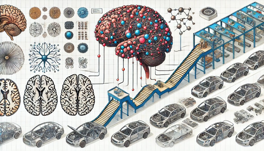
Assembly Line Analogy

Before discussing aspects related to training of Neural Networks, let us look at assembly in a manufacturing unit as rough analogy to understand the concept behind how Neural Network works.

1. Input Layer (Starting Point):
   • Beginning of the assembly line is where raw materials / components (inputs) are introduced. This is like where data enters the Neural Network. In case of car manufacturing, the raw materials such as steel fabrications, tyres, engines may enter the assembly line.
2. Hidden Layers (Stations):
   • Each station on the assembly line represents a hidden layer in the neural network. At each station, workers (neurons) take the incoming materials (data), process them, and pass them on to the next station. (In case of building a car, the first station could frame the body of the car. The second station may install engine, while the third station could add wheels, and the next station may paint).
   • Weights (Tools and Techniques): The tools and techniques used by workers to process the materials represent the weights. They are like the influence each neuron carries.
   • Biases (Adjustments): Just like adjustments made by workers to ensure the specifications of the product, biases adjust the processing to improve accuracy.
   • Activation Function (Quality Check): Each station has a quality check mechanism (activation function) to decide if the processed material should move forward in the assembly line.

Due to highly automated nature of car manufacturing, there may be fewer workers in each station and automation has taken up the role of workers using the tools & applying techniques at each station. Automated process controls handle the movement from one station to the next according to the product specification and quality requirements.

3. Output Layer (End of the Line):
   • The final station on the assembly line is where the fully processed product comes out. The final, complete car rolls off the line, ready to be driven or test driven. This is the output layer where the final prediction or result of Neural Network is produced.

Training the Neural Network

“Cells that fire together, wire together,” is the core idea of how brain learns by adjusting the strength of synapses. When a neuron in brain repeatedly activates another neuron, the synaptic connection between them becomes stronger. Such repeated stimulation of a synapse leads to a long-lasting increase in its strength. Experiences, learning, and memory formation shape neural circuits in the brain. Adopting this idea, Neural Networks are made to learn through training using large data sets representing the context of the problem. Training involves the following steps:

1. Data Preparation:

Gather a dataset relevant to the problem to be solved. Clean the data by removing noise, handling missing values, and normalizing it to a suitable range.

2. Network Initialization:

Choose the type of neural network (see below for popular types of Neural Networks) and define its characteristics such as number of layers, types of layers, number of neurons in each layer. Initialize with random weights for the connections between neurons.

3. Forward Propagation to produce output:

Pass a batch of input data to the first layer. At each layer, compute the output by applying the activation functions to the weighted sum of inputs. Produce the final output of the network.

4. Improving Output:

Compare the network’s output with the actual target values using a loss function. Calculate the loss, which quantifies how far the outputs are from the actual values. Update the weights from the last layer to the first through Back Propagation. Technique called Gradient Descent is used for calculating the loss and updating the weights to minimize the loss.

5. Iteration:

Iterate through forward propagation, loss calculation, and backpropagation until the network’s performance improves. A complete pass through the dataset is referred to as an epoch. Usually, the data is divided into batches, and the weights are updated after processing each batch through multiple epochs.

6. Evaluation:

Evaluate the network on a separate validation data set to check for its performance. Adjust parameters such as number of neurons, number of layers, number of epochs/ data batches etc., and retrain if necessary to improve performance. These parameters are called Hyper Parameters.

Deep learning is the term used for neural networks with many layers to model and understand complex patterns in large datasets.

Popular Neural Networks:

1. Feedforward Neural Networks (FNN): The simplest type of artificial neural network where the information moves in one direction—from input nodes, through hidden nodes to output nodes. They are widely used for pattern recognition.

2. Convolutional Neural Networks (CNN): Primarily used for image and video recognition tasks. They are designed to learn spatial hierarchies of features automatically and adaptively from input images. This works like magnifying glass used to look at small parts of an image to recognize prominent parts. Feature maps of such prominent parts aid in deciding what the image is.

3. Recurrent Neural Networks (RNN): Suitable for sequential data or time series prediction. They have connections that form directed cycles, allowing them to maintain a ‘memory’ of previous inputs. Even in the world of Transformer Networks (see below), RNNs are more effective for applications where data arrives in a continuous stream and decisions need to be made on-the-fly such as Real-Time Speech Recognition and Stock Price prediction.

4. Long Short-Term Memory Networks (LSTM): A type of RNN that can learn long-term dependencies. They are particularly effective for tasks where the context of previous data points is important, such as language modelling. While Transformer Network (see below) does this better, LSTM is preferred for smaller datasets or simpler tasks, as it is easier to implement, and train compared to transformers.

5. Generative Adversarial Networks (GANs): Consist of two neural networks, a generator and a discriminator, which compete against each other. GAN works like iterative constructive criticism of a critic against a creator’s work to improve the creator’s output to make it more realistic. They are used for generating synthetic instances of data, restoring damaged photos by filling up missing parts and for predicting future frames in videos as required in autonomous driving.

6. Transformer Networks: They use mechanisms called attention to weigh the influence of various parts of the input data. Based on the famous research paper ‘Attention Is All You Need,’ from Google researchers, Transformer is the major component of today’s Generative AI – GenAI.

Brain Works or Selfies or Seen-It-Before?

While it is true that many problems solved by traditional statistical machine learning (ML) algorithms such as Selfies and Seen-It-Before, discussed in the previous two parts can also be tackled by neural networks, following are some nuances to consider:

1. Flexibility and Power: Neural networks, especially deep learning models, are highly flexible and powerful. They can model complex, non-linear relationships in data, making them suitable for a wide range of tasks, from image recognition to natural language processing.

2. Data Requirements: Neural networks typically require enormous amounts of data to perform well. Traditional statistical ML algorithms, like linear regression or decision trees is good enough for smaller datasets.

3. Interpretability: Traditional ML algorithms are more interpretable while Neural networks are often considered “black boxes” due to their complexity.

4. Computational Resources: Neural networks, especially deep learning models, require significant computational resources for training. Traditional ML algorithms are usually less resource-intensive and can be cost effective for certain applications.

5. Specific Use Cases: Some problems are better suited to traditional ML algorithms due to their simplicity and efficiency. For example, logistic regression is often used for binary classification tasks, and k-means clustering remains a popular choice for unsupervised learning tasks.

I hope the four parts would have provided a conceptual understanding of essential ML/AI algorithms. We will review how to make an optimum choice of ML/AI algorithms in a later part of this series.